Introduction to ensemble learning

(sources)

Introduction

Ensemble learning?

Combines multiple predictors results to get a better predictor

How to combine?

• averaging for numerical response (regression)
• voting for categorical response (classification)

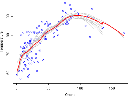
Example: ensemble polynomial regression

[Credit: Tolstoy the Cat CC0 (wikimedia)]

palmerpenguins dataset (Horst, Hill, and Gorman 2020)

# A tibble: 6 × 8
  species island    bill_length_mm bill_depth_mm flipper_length_mm body_mass_g
  <fct>   <fct>              <dbl>         <dbl>             <int>       <int>
1 Adelie  Torgersen           39.1          18.7               181        3750
2 Adelie  Torgersen           39.5          17.4               186        3800
3 Adelie  Torgersen           40.3          18                 195        3250
4 Adelie  Torgersen           NA            NA                  NA          NA
5 Adelie  Torgersen           36.7          19.3               193        3450
6 Adelie  Torgersen           39.3          20.6               190        3650
# ℹ 2 more variables: sex <fct>, year <int>

   Adelie Chinstrap    Gentoo 
      152        68       124 

Pre-processing

• remove missing values

library(tidyr)
library(dplyr)

penguins <- penguins %>% drop_na()

• split in train and test set

set.seed(1234)
sample <- sample(c(TRUE, FALSE), nrow(penguins), replace=TRUE, prob=c(0.7,0.3))

train_df <- penguins[sample,]
test_df <- penguins[!sample,]

• extract response (species) and covariates (bill_length_mm, bill_depth_mm, flipper_length_mm, body_mass_g)

X_train <- train_df %>% 
    dplyr::select(bill_length_mm, bill_depth_mm, flipper_length_mm, body_mass_g) %>% as.matrix()
y_train <- train_df %>% select(species) %>% pull()

X_test <- test_df %>%
    dplyr::select(bill_length_mm, bill_depth_mm, flipper_length_mm, body_mass_g) %>% as.matrix()
y_test <- test_df %>% select(species) %>% pull()

• scale data

X_train <- scale(X_train)
X_train_mean <- attributes(X_train)$`scaled:center`
X_train_sd <- attributes(X_train)$`scaled:scale`
X_test <- scale(X_test, center = X_train_mean, scale = X_train_sd)

# remerge data.frame
train_df <- cbind(
    as.data.frame(X_train), train_df %>% select(species, year, sex, island))
test_df <- cbind(
    as.data.frame(X_test), test_df %>% select(species, year, sex, island))

Bagging

Bagging = bootstrap aggregating (Breiman 1996)

• Train multiple (weak) predictors on data boostrap resamples

Variation: train the predictors on data subsamples (and keep unused data to compute out-of-bag error)

Bagging procedure

[Credit: Sirakorn CC BY-SA 4.0 (wikimedia)]

Boostrap (Efron 1979)

Standard sampling

[Credit: Trist’n Joseph]

Boostrap multiple sampling (sampling with replacement)

[Credit: Trist’n Joseph]

Bagging pros ans cons

Advantages:

• Aggregation of many weak predictors outperforms a single predictor in term of accuracy
• Reduce overfitting (better generalization)
• Can be performed in parallel

Disadvantages:

• For weak learner with high bias, bagging results will also be biased
• Loss of interpretability for the model
• Potentially computationally expensive depending on the data set

Boosting

Boosting meta-algorithm (Schapire 1990)

• Iteratively train week predictors
• Weight data depending on previous predictor error (to focus on data with higher error rate in next predictor)

⟶ several algorithms (AdaBoost, LPBoost, TotalBoost, BrownBoost, xgboost, MadaBoost, LogitBoost, etc.)

Boosting procedure

[Credit: Sirakorn CC BY-SA 4.0 (wikimedia)]

Random forest

Decision tree

Classification and Regression Tree (CART): Breiman et al. (1984)

• build a decision tree to split the training data set by setting threshold on covariates

• use average/voting in the leaves to predict the response for regression/classification (resp.)

Example of regression tree

species ~ bill_length_mm + bill_depth_mm + flipper_length_mm + 
    body_mass_g + sex

library(rpart)
library(rpart.plot)

tree <- rpart(
    species ~ . - island - year,
    data = train_df,
    method="class",
    control=rpart.control(minsplit=5,cp=0)
)
# plotcp(tree)

prp(tree,extra=1)

CART algorithm illustration

species ~ bill_length_mm + bill_depth_mm

Data: ::: {.cell} ::: {.cell-output-display} ::: :::

Step 1: bill_length_mm < -0.11 ? ::: {.cell} ::: {.cell-output-display} ::: :::

Step 2: bill_length_mm < -0.11 and bill_depth_mm >= -1.1? ::: {.cell} ::: {.cell-output-display} ::: :::

Step 3: bill_length_mm >= -0.11 and bill_depth_mm >= -0.45? ::: {.cell} ::: {.cell-output-display} ::: ::: \[\vdots\]

Random forest (Breiman 2001)

• aggregate multiple decision tree predictors
• bagging + random selection of covariates to build the decision trees

Random forest procedure

Decision tree and random forest [Credit: CollaborativeGeneticist CC BY-SA 4.0 (wikimedia)]

Illustration

Problem

Prediction of the penguins species using

• bill_length_mm
• bill_depth_mm
• flipper_length_mm
• body_mass_g
• sex

Bag of trees vs Random forest

# bag of tree
bagging_tree <- function(
        train_df, test_df, n_boot = 100) {
    
    boot_res <- Reduce("rbind", lapply(
        1:n_boot,
        function(id) {
            
            boot_samp <- sample(
                1:nrow(X_train),
                size=round(nrow(X_train)),
                replace=TRUE
            )
            
            tmp_mod <- rpart(
                species ~ . - island - year,
                data = train_df[boot_samp,],
                method="class",
                control=rpart.control(minsplit=5,cp=0)
            )
            
            tmp_pred <- predict(tmp_mod, test_df, type = "class")
            return(as.character(tmp_pred))
        }
    ))
    
    pred_res <- apply(
        boot_res, 2, 
        function(boot_pred) {
            tmp_count <- table(boot_pred)
            names(tmp_count)[which.max(tmp_count)]
        }
    )
    
    indiv_tree_error_df <- apply(
        boot_res, 1, 
        function(boot_pred) {
            return(mean(boot_pred != test_df$species))
        }
    )
    
    indiv_tree_error_av <- mean(indiv_tree_error_df)
    indiv_tree_error_sd <- sd(indiv_tree_error_df)
    
    bag_tree_error <- mean(pred_res != test_df$species)
    
    return(lst(indiv_tree_error_av, indiv_tree_error_sd,  bag_tree_error))
}

bag_tree_res <- bagging_tree(train_df, test_df, n_boot = 100)

library(randomForest)
rf <- randomForest(
    species ~ . - island - year, data=train_df, proximity=TRUE
)

rf_pred <- predict(rf, test_df, type = "response")
rf_error <- mean(rf_pred != test_df$species)

Results

• Bag of tree: ::: {.cell} ::: {.cell-output .cell-output-stdout}

$indiv_tree_error_av
[1] 0.06191489

$indiv_tree_error_sd
[1] 0.02086317

$bag_tree_error
[1] 0.04255319

::: :::

• Random forest: ::: {.cell} ::: {.cell-output .cell-output-stdout}

[1] 0.03191489

::: :::

Application

scClassify: multiscale classification of single cell gene expression data (Lin et al. 2020)

• hierarchical clustering

• ensemble classification for cell type prediction inside each cluster

scClassify: the model

(Credit: Lin et al. 2020)

scClassify: the results

(Credit: Lin et al. 2020)

Outro

Take home message

• Ensemble methods: strength in number (for weak predictors)

• Avoid hyper-parameter calibration: aggregate predictors with different hyper-parameter values

References

References

Breiman, Leo. 1996. “Bagging Predictors.” Machine Learning 24 (2): 123–40. https://doi.org/10.1007/BF00058655.

———. 2001. “Random Forests.” Machine Learning 45 (1): 5–32. http://link.springer.com/article/10.1023/A:1010933404324.

Breiman, Leo, Jerome Friedman, Charles J. Stone, and R. A. Olshen. 1984. Classification and Regression Trees. New Ed. Boca Raton: Chapman; Hall/CRC.

Efron, B. 1979. “Bootstrap Methods: Another Look at the Jackknife.” The Annals of Statistics 7 (1): 1–26. https://doi.org/10.1214/aos/1176344552.

Horst, Allison Marie, Alison Presmanes Hill, and Kristen B Gorman. 2020. Palmerpenguins: Palmer Archipelago (Antarctica) Penguin Data. https://doi.org/10.5281/zenodo.3960218.

Lin, Yingxin, Yue Cao, Hani Jieun Kim, Agus Salim, Terence P Speed, David M Lin, Pengyi Yang, and Jean Yee Hwa Yang. 2020. “scClassify: Sample Size Estimation and Multiscale Classification of Cells Using Single and Multiple Reference.” Molecular Systems Biology 16 (6): e9389. https://doi.org/10.15252/msb.20199389.

Schapire, Robert E. 1990. “The Strength of Weak Learnability.” Machine Learning 5 (2): 197–227. https://doi.org/10.1007/BF00116037.